Start Here: datascience Tutorial
This is a brief introduction to the functionality in
datascience. For a complete reference guide, please see
Tables (datascience.tables).
For other useful tutorials and examples, see:
Getting Started
The most important functionality in the package is is the Table
class, which is the structure used to represent columns of data. First, load
the class:
In [1]: from datascience import Table
In the IPython notebook, type Table. followed by the TAB-key to see a list
of members.
Note that for the Data Science 8 class we also import additional packages and settings for all assignments and labs. This is so that plots and other available packages mirror the ones in the textbook more closely. The exact code we use is:
# HIDDEN

import matplotlib
matplotlib.use('Agg')
from datascience import Table
%matplotlib inline
import matplotlib.pyplot as plt
import numpy as np
plt.style.use('fivethirtyeight')
In particular, the lines involving matplotlib allow for plotting within the
IPython notebook.
Creating a Table
A Table is a sequence of labeled columns of data.
A Table can be constructed from scratch by extending an empty table with columns.
In [2]: t = Table().with_columns(
   ...:     'letter', ['a', 'b', 'c', 'z'],
   ...:     'count',  [  9,   3,   3,   1],
   ...:     'points', [  1,   2,   2,  10],
   ...: )
   ...:

In [3]: print(t)
letter | count | points
a      | 9     | 1
b      | 3     | 2
c      | 3     | 2
z      | 1     | 10
More often, a table is read from a CSV file (or an Excel spreadsheet). Here’s the content of an example file:
In [4]: cat sample.csv
x,y,z
1,10,100
2,11,101
3,12,102
And this is how we load it in as a Table using
read_table():
In [5]: Table.read_table('sample.csv')
Out[5]:
x    | y    | z
1    | 10   | 100
2    | 11   | 101
3    | 12   | 102
CSVs from URLs are also valid inputs to
read_table():
In [6]: Table.read_table('https://www.inferentialthinking.com/data/sat2014.csv')
Out[6]:
State        | Participation Rate | Critical Reading | Math | Writing | Combined
North Dakota | 2.3                | 612              | 620  | 584     | 1816
Illinois     | 4.6                | 599              | 616  | 587     | 1802
Iowa         | 3.1                | 605              | 611  | 578     | 1794
South Dakota | 2.9                | 604              | 609  | 579     | 1792
Minnesota    | 5.9                | 598              | 610  | 578     | 1786
Michigan     | 3.8                | 593              | 610  | 581     | 1784
Wisconsin    | 3.9                | 596              | 608  | 578     | 1782
Missouri     | 4.2                | 595              | 597  | 579     | 1771
Wyoming      | 3.3                | 590              | 599  | 573     | 1762
Kansas       | 5.3                | 591              | 596  | 566     | 1753
... (41 rows omitted)
It’s also possible to add columns from a dictionary, but this option is discouraged because dictionaries do not preserve column order.
In [7]: t = Table().with_columns({
   ...:     'letter': ['a', 'b', 'c', 'z'],
   ...:     'count':  [  9,   3,   3,   1],
   ...:     'points': [  1,   2,   2,  10],
   ...: })
   ...:

In [8]: print(t)
letter | count | points
a      | 9     | 1
b      | 3     | 2
c      | 3     | 2
z      | 1     | 10
Accessing Values
To access values of columns in the table, use
column(), which takes a column label or index
and returns an array. Alternatively, columns()
returns a list of columns (arrays).
In [9]: t
Out[9]:
letter | count | points
a      | 9     | 1
b      | 3     | 2
c      | 3     | 2
z      | 1     | 10

In [10]: t.column('letter')
Out[10]:
array(['a', 'b', 'c', 'z'],
      dtype='<U1')

In [11]: t.column(1)
Out[11]: array([9, 3, 3, 1])
You can use bracket notation as a shorthand for this method:
In [12]: t['letter'] # This is a shorthand for t.column('letter')
Out[12]:
array(['a', 'b', 'c', 'z'],
      dtype='<U1')

In [13]: t[1]        # This is a shorthand for t.column(1)
Out[13]: array([9, 3, 3, 1])
To access values by row, row() returns a
row by index. Alternatively, rows() returns an
list-like Rows object that contains
tuple-like Row objects.
In [14]: t.rows
Out[14]:
Rows(letter | count | points
a      | 9     | 1
b      | 3     | 2
c      | 3     | 2
z      | 1     | 10)

In [15]: t.rows[0]
Out[15]: Row(letter='a', count=9, points=1)

In [16]: t.row(0)
Out[16]: Row(letter='a', count=9, points=1)

In [17]: second = t.rows[1]

In [18]: second
Out[18]: Row(letter='b', count=3, points=2)

In [19]: second[0]
Out[19]: 'b'

In [20]: second[1]
Out[20]: 3
To get the number of rows, use num_rows.
In [21]: t.num_rows
Out[21]: 4
Manipulating Data
Here are some of the most common operations on data. For the rest, see the reference (Tables (datascience.tables)).
Adding a column with with_column():
In [22]: t
Out[22]:
letter | count | points
a      | 9     | 1
b      | 3     | 2
c      | 3     | 2
z      | 1     | 10

In [23]: t.with_column('vowel?', ['yes', 'no', 'no', 'no'])
Out[23]:
letter | count | points | vowel?
a      | 9     | 1      | yes
b      | 3     | 2      | no
c      | 3     | 2      | no
z      | 1     | 10     | no

In [24]: t # .with_column returns a new table without modifying the original
Out[24]:
letter | count | points
a      | 9     | 1
b      | 3     | 2
c      | 3     | 2
z      | 1     | 10

In [25]: t.with_column('2 * count', t['count'] * 2) # A simple way to operate on columns
Out[25]:
letter | count | points | 2 * count
a      | 9     | 1      | 18
b      | 3     | 2      | 6
c      | 3     | 2      | 6
z      | 1     | 10     | 2
Selecting columns with select():
In [26]: t.select('letter')
Out[26]:
letter
a
b
c
z

In [27]: t.select(['letter', 'points'])
Out[27]:
letter | points
a      | 1
b      | 2
c      | 2
z      | 10
Renaming columns with relabeled():
In [28]: t
Out[28]:
letter | count | points
a      | 9     | 1
b      | 3     | 2
c      | 3     | 2
z      | 1     | 10

In [29]: t.relabeled('points', 'other name')
Out[29]:
letter | count | other name
a      | 9     | 1
b      | 3     | 2
c      | 3     | 2
z      | 1     | 10

In [30]: t
Out[30]:
letter | count | points
a      | 9     | 1
b      | 3     | 2
c      | 3     | 2
z      | 1     | 10

In [31]: t.relabeled(['letter', 'count', 'points'], ['x', 'y', 'z'])
Out[31]:
x    | y    | z
a    | 9    | 1
b    | 3    | 2
c    | 3    | 2
z    | 1    | 10
Selecting out rows by index with take() and
conditionally with where():
In [32]: t
Out[32]:
letter | count | points
a      | 9     | 1
b      | 3     | 2
c      | 3     | 2
z      | 1     | 10

In [33]: t.take(2) # the third row
Out[33]:
letter | count | points
c      | 3     | 2

In [34]: t.take[0:2] # the first and second rows
Out[34]:
letter | count | points
a      | 9     | 1
b      | 3     | 2
In [35]: t.where('points', 2) # rows where points == 2
Out[35]:
letter | count | points
b      | 3     | 2
c      | 3     | 2

In [36]: t.where(t['count'] < 8) # rows where count < 8
Out[36]:
letter | count | points
b      | 3     | 2
c      | 3     | 2
z      | 1     | 10

In [37]: t['count'] < 8 # .where actually takes in an array of booleans
Out[37]: array([False,  True,  True,  True], dtype=bool)

In [38]: t.where([False, True, True, True]) # same as the last line
Out[38]:
letter | count | points
b      | 3     | 2
c      | 3     | 2
z      | 1     | 10
Operate on table data with sort(),
group(), and
pivot()
In [39]: t
Out[39]:
letter | count | points
a      | 9     | 1
b      | 3     | 2
c      | 3     | 2
z      | 1     | 10

In [40]: t.sort('count')
Out[40]:
letter | count | points
z      | 1     | 10
b      | 3     | 2
c      | 3     | 2
a      | 9     | 1

In [41]: t.sort('letter', descending = True)
Out[41]:
letter | count | points
z      | 1     | 10
c      | 3     | 2
b      | 3     | 2
a      | 9     | 1
# You may pass a reducing function into the collect arg
# Note the renaming of the points column because of the collect arg
In [42]: t.select(['count', 'points']).group('count', collect=sum)
Out[42]:
count | points sum
1     | 10
3     | 4
9     | 1
In [43]: other_table = Table().with_columns(
   ....:     'mar_status',  ['married', 'married', 'partner', 'partner', 'married'],
   ....:     'empl_status', ['Working as paid', 'Working as paid', 'Not working',
   ....:                     'Not working', 'Not working'],
   ....:     'count',       [1, 1, 1, 1, 1])
   ....:

In [44]: other_table
Out[44]:
mar_status | empl_status     | count
married    | Working as paid | 1
married    | Working as paid | 1
partner    | Not working     | 1
partner    | Not working     | 1
married    | Not working     | 1

In [45]: other_table.pivot('mar_status', 'empl_status', 'count', collect=sum)
Out[45]:
empl_status     | married | partner
Not working     | 1       | 2
Working as paid | 2       | 0
Visualizing Data
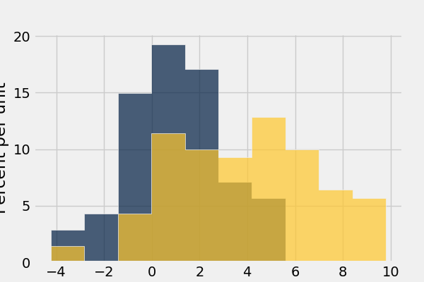
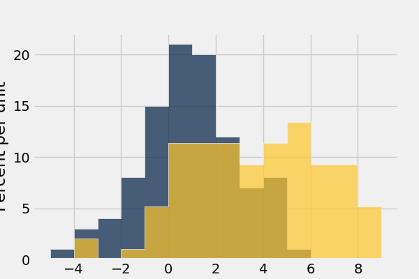
We’ll start with some data drawn at random from two normal distributions:
In [46]: normal_data = Table().with_columns(
   ....:     'data1', np.random.normal(loc = 1, scale = 2, size = 100),
   ....:     'data2', np.random.normal(loc = 4, scale = 3, size = 100))
   ....:

In [47]: normal_data
Out[47]:
data1      | data2
-1.20283   | -0.125011
-0.0747679 | 1.74108
2.60632    | 8.0518
1.71311    | 1.01439
3.01951    | 1.69442
2.22393    | 6.00219
0.53912    | 6.54448
3.33215    | 2.80953
3.52172    | 4.82624
3.54184    | 1.39129
... (90 rows omitted)
Draw histograms with hist():
In [48]: normal_data.hist()
In [49]: normal_data.hist(bins = range(-5, 10))

In [50]: normal_data.hist(bins = range(-5, 10), overlay = True)
Draw grouped histograms with the group argument:
In [51]: grouped = Table().with_columns(
   ....:     'value', np.random.normal(size=100),
   ....:     'group', np.random.choice(['A', 'B'], size=100)
   ....: )
   ....:

In [52]: grouped.hist('value', group='group')
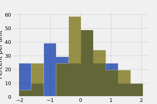
Note: group cannot be used together with bin_column, and does not support multiple histogram columns.
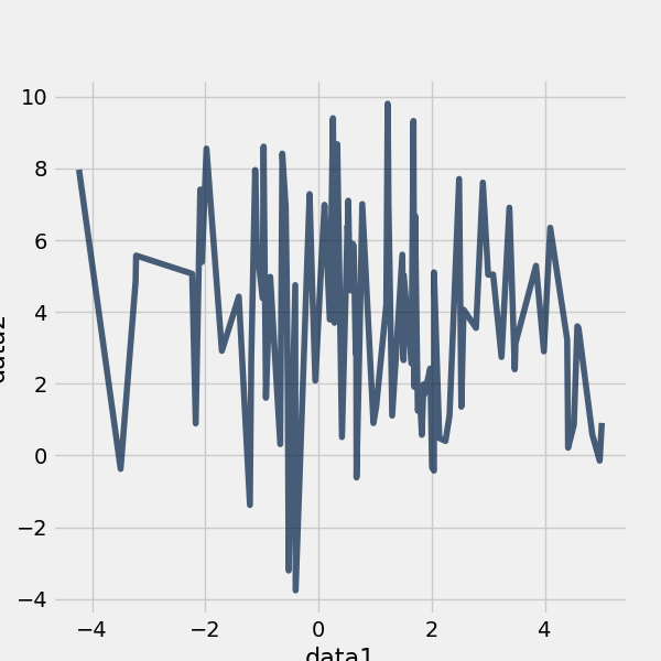
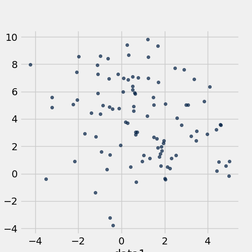
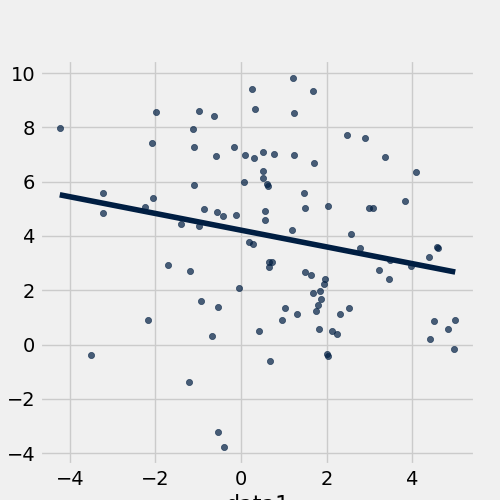
If we treat the normal_data table as a set of x-y points, we can
plot() and
scatter():
In [53]: normal_data.sort('data1').plot('data1') # Sort first to make plot nicer
In [54]: normal_data.scatter('data1')
In [55]: normal_data.scatter('data1', fit_line = True)
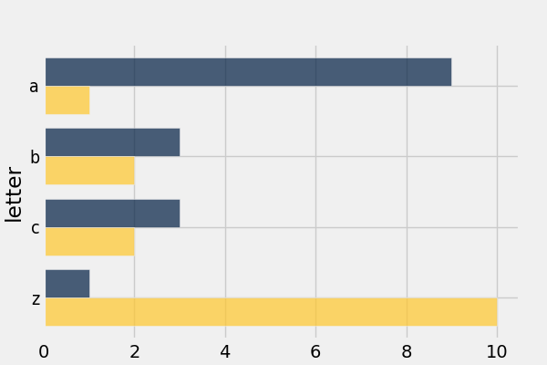
Use barh() to display categorical data.
In [56]: t
Out[56]:
letter | count | points
a      | 9     | 1
b      | 3     | 2
c      | 3     | 2
z      | 1     | 10

In [57]: t.barh('letter')
Exporting
Exporting to CSV is the most common operation and can be done by first
converting to a pandas dataframe with to_df():
In [58]: normal_data
Out[58]:
data1      | data2
-1.20283   | -0.125011
-0.0747679 | 1.74108
2.60632    | 8.0518
1.71311    | 1.01439
3.01951    | 1.69442
2.22393    | 6.00219
0.53912    | 6.54448
3.33215    | 2.80953
3.52172    | 4.82624
3.54184    | 1.39129
... (90 rows omitted)

# index = False prevents row numbers from appearing in the resulting CSV
In [59]: normal_data.to_df().to_csv('normal_data.csv', index = False)
An Example
We’ll recreate the steps in Chapter 12 of the textbook to see if there is a significant difference in birth weights between smokers and non-smokers using a bootstrap test.
For more examples, check out the TableDemos repo.
From the text:
The table
babycontains data on a random sample of 1,174 mothers and their newborn babies. The columnBirth Weightcontains the birth weight of the baby, in ounces;Gestational Daysis the number of gestational days, that is, the number of days the baby was in the womb. There is also data on maternal age, maternal height, maternal pregnancy weight, and whether or not the mother was a smoker.
In [60]: baby = Table.read_table('https://www.inferentialthinking.com/data/baby.csv')

In [61]: baby # Let's take a peek at the table
Out[61]:
Birth Weight | Gestational Days | Maternal Age | Maternal Height | Maternal Pregnancy Weight | Maternal Smoker
120          | 284              | 27           | 62              | 100                       | False
113          | 282              | 33           | 64              | 135                       | False
128          | 279              | 28           | 64              | 115                       | True
108          | 282              | 23           | 67              | 125                       | True
136          | 286              | 25           | 62              | 93                        | False
138          | 244              | 33           | 62              | 178                       | False
132          | 245              | 23           | 65              | 140                       | False
120          | 289              | 25           | 62              | 125                       | False
143          | 299              | 30           | 66              | 136                       | True
140          | 351              | 27           | 68              | 120                       | False
... (1164 rows omitted)

# Select out columns we want.
In [62]: smoker_and_wt = baby.select(['Maternal Smoker', 'Birth Weight'])

In [63]: smoker_and_wt
Out[63]:
Maternal Smoker | Birth Weight
False           | 120
False           | 113
True            | 128
True            | 108
False           | 136
False           | 138
False           | 132
False           | 120
True            | 143
False           | 140
... (1164 rows omitted)
Let’s compare the number of smokers to non-smokers.
In [64]: smoker_and_wt.select('Maternal Smoker').group('Maternal Smoker')
Out[64]:
Maternal Smoker | count
False           | 715
True            | 459
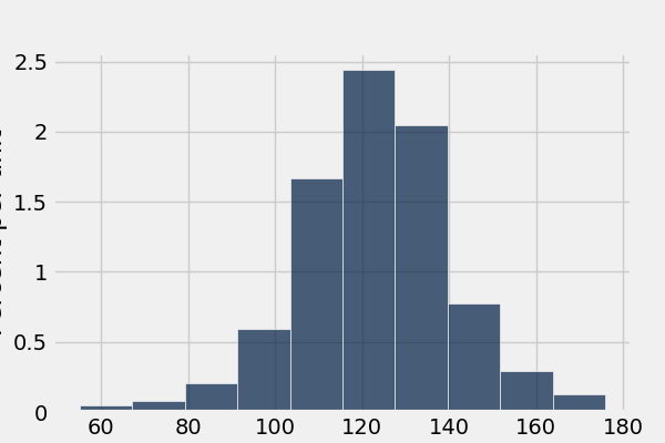
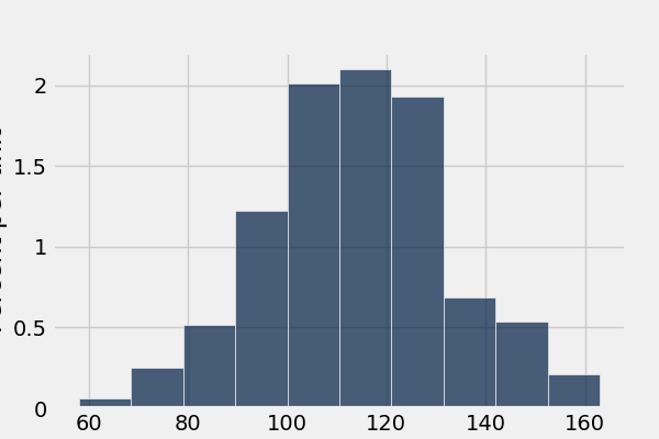
We can also compare the distribution of birthweights between smokers and non-smokers.
# Non smokers
# We do this by grabbing the rows that correspond to mothers that don't
# smoke, then plotting a histogram of just the birthweights.
In [65]: smoker_and_wt.where('Maternal Smoker', 0).select('Birth Weight').hist()

# Smokers
In [66]: smoker_and_wt.where('Maternal Smoker', 1).select('Birth Weight').hist()
What’s the difference in mean birth weight of the two categories?
In [67]: nonsmoking_mean = smoker_and_wt.where('Maternal Smoker', 0).column('Birth Weight').mean()

In [68]: smoking_mean = smoker_and_wt.where('Maternal Smoker', 1).column('Birth Weight').mean()

In [69]: observed_diff = nonsmoking_mean - smoking_mean

In [70]: observed_diff
Out[70]: 9.2661425720249184
Let’s do the bootstrap test on the two categories.
In [71]: num_nonsmokers = smoker_and_wt.where('Maternal Smoker', 0).num_rows

In [72]: def bootstrap_once():
   ....:     """
   ....:     Computes one bootstrapped difference in means.
   ....:     The table.sample method lets us take random samples.
   ....:     We then split according to the number of nonsmokers in the original sample.
   ....:     """
   ....:     resample = smoker_and_wt.sample(with_replacement = True)
   ....:     bootstrap_diff = resample.column('Birth Weight')[:num_nonsmokers].mean() - \
   ....:         resample.column('Birth Weight')[num_nonsmokers:].mean()
   ....:     return bootstrap_diff
   ....:

In [73]: repetitions = 1000

In [74]: bootstrapped_diff_means = np.array(
   ....:     [ bootstrap_once() for _ in range(repetitions) ])
   ....:

In [75]: bootstrapped_diff_means[:10]
Out[75]:
array([-0.33552112, -0.98629736,  0.11038896,  0.72915886,  0.10513887,
        0.40491491, -0.74449777,  0.3660862 , -1.03620519, -1.39999086])

In [76]: num_diffs_greater = (abs(bootstrapped_diff_means) > abs(observed_diff)).sum()

In [77]: p_value = num_diffs_greater / len(bootstrapped_diff_means)

In [78]: p_value
Out[78]: 0.0
Drawing Maps
The main class in the maps module is the Map class. In this code we create a default Map. Maps can be displayed or converted to html.
In [79]: from datascience.maps import Map    # import the Map class

In [80]: default_map = Map()                 # generate a default Map

In [81]: default_map.show()                  # display the Map
<IPython.core.display.HTML object>

In [82]: html = default_map.as_html()        # generate the html

In [83]: with open('map.html', 'w') as f:    # make a file to store the html
   ....:     f.write(html)                   # write the html to the file
   ....:
The maps modules also allows you to make custom maps with markers, circles and regions.
In [84]: from datascience.maps import Map, Marker, Circle, Region            # import the Map, Marker, Circle and Region class

# generates markers with custom sets of coordinates, colors and popups
In [85]: marker1 = Marker(37.372, -121.758, color="green", popup="My green marker")

In [86]: marker2 = Marker(37.572, -121.758, color="orange", popup="My orange marker")

# generates a circle with a custom set of coordinates, color and popup
In [87]: circle = Circle(37.5, -122, color="red", area=1000, popup="My Circle")

# make a geojson object which is needed when making a region
In [88]: geojson = {
   ....:   "type": "Feature",
   ....:   "geometry": {
   ....:     "type": "Polygon",
   ....:     "coordinates": [                                                # specifies the coordinates
   ....:         [[-121,37],[-121.5,37],[-121.5,37.5],[-121,37.5],[-121,37]] # these coordinates make a rectangle
   ....:     ]
   ....:   }
   ....: }
   ....:

# make a region with your geojson object
In [89]: region = Region(geojson)

# Initialize the map
In [90]: custom_map = Map(features=[marker1, marker2, circle, region],       # specifies the features
   ....:          width=800,                                                 # specifies a custom width
   ....:          height=600                                                 # specifies a custom height
   ....:                 )
   ....:

In [91]: custom_map.show()                                                   # display the map
<IPython.core.display.HTML object>