import matplotlib
from datascience import *
%matplotlib inline
import matplotlib.pyplot as plots
import numpy as np
plots.style.use('fivethirtyeight')
# Some functions for plotting. You don't have to understand how any
# of the functions in this cell work, since they use things we
# haven't learned about in Data 8.
def resize_window(lim=3.5):
plots.xlim(-lim, lim)
plots.ylim(-lim, lim)
def draw_line(slope=0, intercept=0, x=make_array(-4, 4), color='#44AA00'):
y = x*slope + intercept
plots.plot(x, y, color=color, lw=3)
def draw_vertical_line(x_position, color='black'):
x = make_array(x_position, x_position)
y = make_array(-4, 4)
plots.plot(x, y, color=color, lw=3)
def make_correlated_data(r):
x = np.random.normal(0, 1, 1000)
z = np.random.normal(0, 1, 1000)
y = r*x + (np.sqrt(1-r**2))*z
return x, y
def r_scatter(r):
"""Generate a scatter plot with a correlation approximately r"""
plots.figure(figsize=(5,5))
x, y = make_correlated_data(r)
plots.scatter(x, y, color='darkblue', s=20)
plots.xlim(-4, 4)
plots.ylim(-4, 4)
def r_table(r):
"""
Generate a table of 1000 data points with a correlation approximately r
"""
np.random.seed(8)
x, y = make_correlated_data(r)
return Table().with_columns('x', x, 'y', y)Functions from previous lectures
def standard_units(x):
    "Convert any array of numbers to standard units."
    return (x - np.average(x)) / np.std(x)
def correlation(t, x, y):
"""t is a table; x and y are column labels"""
x_in_standard_units = standard_units(t.column(x))
y_in_standard_units = standard_units(t.column(y))
return np.average(x_in_standard_units * y_in_standard_units)Nonlinearity
new_x = np.arange(-4, 4.1, 0.5)
nonlinear = Table().with_columns(
        'x', new_x,
        'y', new_x**2
    )
nonlinear.scatter('x', 'y', s=30, color='r')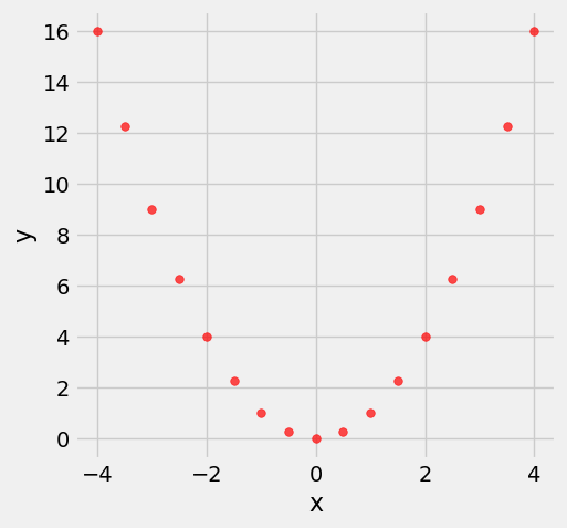
correlation(nonlinear, 'x', 'y')0.0Prediction Lines
example = r_table(0.99)
example.show(3)
Loading...
example.scatter('x', 'y')
resize_window()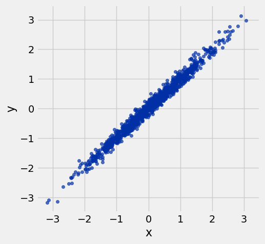
def nn_prediction_example(x_val):
    """ Predicts y-value for x based on the example table """
    neighbors = example.where('x', are.between(x_val - .25, x_val + .25))
return np.mean(neighbors.column('y')) nn_prediction_example(-2.25)-2.1476337989800527example = example.with_columns(
'Predicted y',
example.apply(nn_prediction_example, 'x'))example.scatter('x')
resize_window()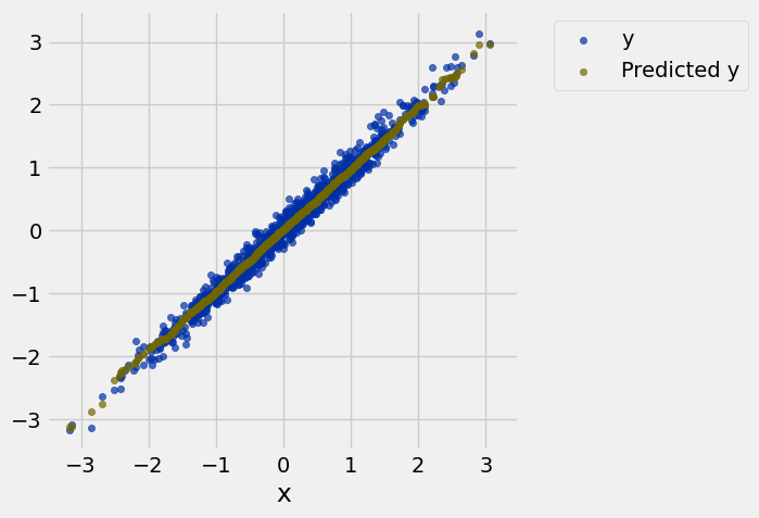
example.scatter('x')
draw_line(slope=1)
resize_window()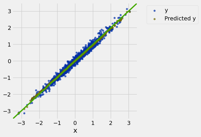
r = 0
example = r_table(0)
example.scatter('x', 'y')
resize_window()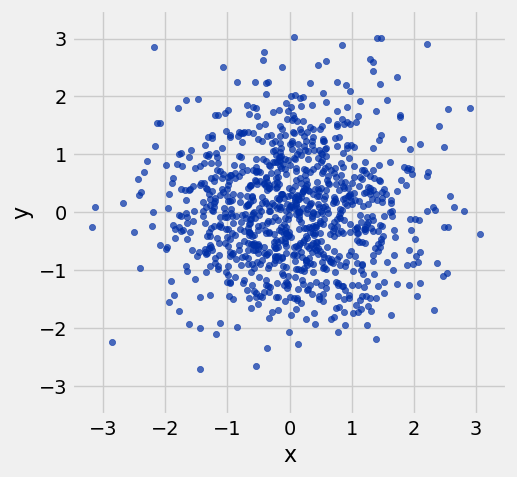
example = example.with_columns(
    'Predicted y',
    example.apply(nn_prediction_example, 'x'))
example.scatter('x')
draw_line(slope=0)
resize_window()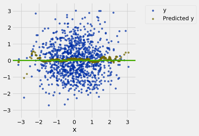
r = 0.5
example = r_table(0.5)
example.scatter('x', 'y')
resize_window()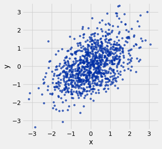
example = r_table(0.5)
example.scatter('x', 'y')
resize_window()
draw_vertical_line(1.5)
draw_line(slope=1, intercept=0, color='red')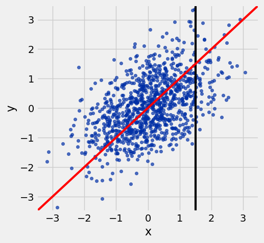
example = example.with_column('Predicted y', example.apply(nn_prediction_example, 'x'))
example.scatter('x')
draw_line(slope=1, color='red')
draw_vertical_line(1.5)
resize_window()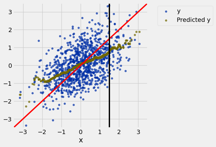
example.scatter('x')
draw_line(slope=1, intercept=0, color='red')
draw_line(slope=0.5, intercept=0)
resize_window()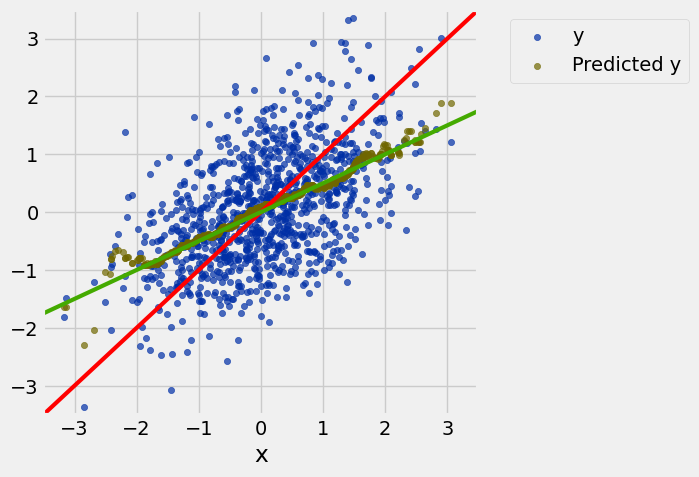
r = 0.7
example = r_table(0.7)
example = example.with_column('Predicted y', example.apply(nn_prediction_example, 'x'))
example.scatter('x')
draw_line(slope=1, intercept=0, color='red')
draw_line(slope=0.7, intercept=0)
resize_window()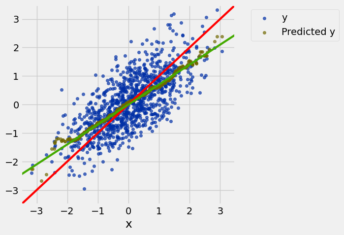
Linear regression: defining the line
def slope(t, x, y):
    """Computes the slope of the regression line"""
    r = correlation(t, x, y)
    y_sd = np.std(t.column(y))
    x_sd = np.std(t.column(x))
    return r * y_sd / x_sd
def intercept(t, x, y):
"""Computes the intercept of the regression line"""
x_mean = np.mean(t.column(x))
y_mean = np.mean(t.column(y))
return y_mean - slope(t, x, y)*x_meanexample = r_table(0.5)
slope(example, 'x', 'y')0.50226382816259152Heights Data and Regression Line
# Note: Child heights are the **adult** heights of children in a family
families = Table.read_table('family_heights.csv')
parent_avgs = (families.column('father') + families.column('mother'))/2
heights = Table().with_columns(
    'Parent Average', parent_avgs,
    'Child', families.column('child'),
)
heights.show(5)
Loading...
def nn_prediction_height(p_avg):
    """Predict the height of a child whose parents have a parent average height of p_avg.

    The prediction is the average height of the children whose parent average height is
    in the range p_avg plus or minus 0.5.
    """

    close_points = heights.where('Parent Average', are.between(p_avg-0.5, p_avg + 0.5))
    return np.average(close_points.column('Child'))
heights_with_predictions = heights.with_column(
'Nearest neighbor prediction',
heights.apply(nn_prediction_height, 'Parent Average'))
heights_with_predictions.show(5)Loading...
heights_with_predictions.scatter('Parent Average')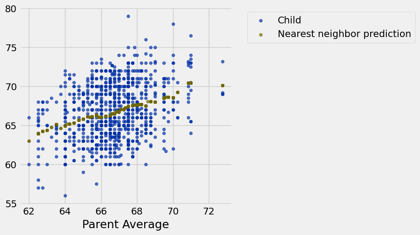
predicted_heights_slope = slope(heights, 'Parent Average', 'Child')
predicted_heights_intercept = intercept(heights, 'Parent Average', 'Child')
[predicted_heights_slope, predicted_heights_intercept]
[0.66449526235258838, 22.461839955758798]heights_with_predictions.scatter('Parent Average')
draw_line(slope=predicted_heights_slope,
intercept=predicted_heights_intercept,
x=heights.column('Parent Average'))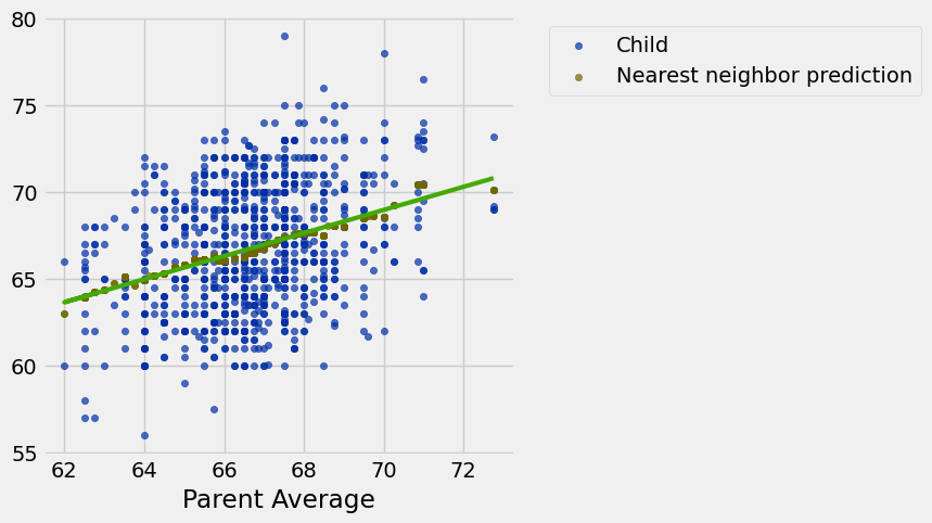
Discussion Question: Exam Score Prediction
# X-axis: midterm scores
midterm_mean = 70
midterm_sd = 10

# Y-axis: final scores
final_mean = 50
final_sd = 12

# Correlation (relates X to Y values)
corr = 0.75

# X value
midterm_student = 90
midterm_student_su = (midterm_student - midterm_mean) / midterm_sd
midterm_student_su2.0final_student_su = midterm_student_su * corr
final_student_su1.5final_student = final_student_su * final_sd + final_mean
final_student68.0