from datascience import *
import numpy as np

%matplotlib inline
import matplotlib.pyplot as plots
plots.style.use('fivethirtyeight')
The GSI’s Defense
scores = Table.read_table('scores_by_section.csv')
scores
Loading...
max(scores.column('Midterm'))25min(scores.column('Midterm'))0scores.group('Section')Loading...
scores.group('Section', np.average).show()Loading...
observed_average = 13.6667 # Null hypothesis: The midterm scores for section 3 are like a
# random draw of 27 students from the course
# Alternative hyp: The midterm scores for section 3 are too low
# to be explained well by randomness alone.
random_sample = scores.sample(27, with_replacement=False)
random_sampleLoading...
np.average(random_sample.column('Midterm'))16.185185185185187# Simulate one value of the test statistic
# under the hypothesis that the section is like a random sample from the class
def random_sample_midterm_avg():
random_sample = scores.sample(27, with_replacement = False)
return np.average(random_sample.column('Midterm'))# Simulate 100,000 copies of the test statistic
sample_averages = make_array()
for i in np.arange(100000):
sample_averages = np.append(sample_averages, random_sample_midterm_avg()) Our Decision
# Compare the simulated distribution of the statistic
# and the actual observed statistic
averages_tbl = Table().with_column('Random Sample Average', sample_averages)
averages_tbl.hist(bins = 20)
plots.scatter(observed_average, -0.01, color='red', s=120);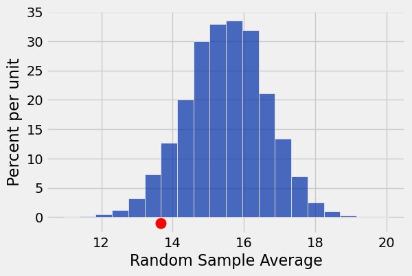
Approach 1
# (1) Calculate the p-value: simulation area beyond observed value
np.count_nonzero(sample_averages <= observed_average) / 100000
# (2) See if this is less than 5%0.05717Approach 2
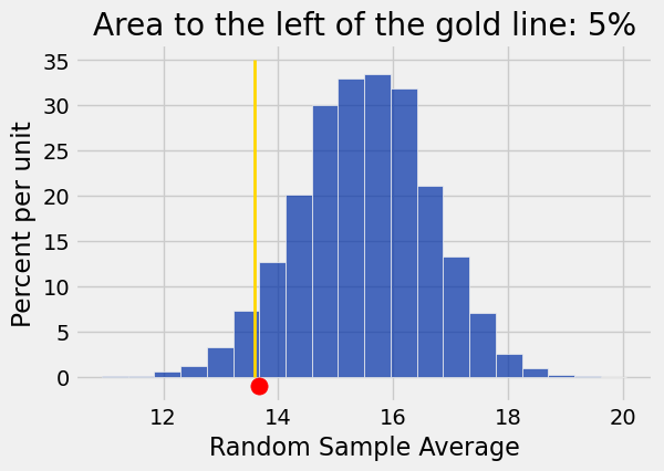
five_percent_point = averages_tbl.sort(0).column(0).item(round(len(sample_averages) * 0.05))
five_percent_point13.592592592592593# (2) See if this value is greater than observed value
observed_average13.6667Visual Representation
averages_tbl.hist(bins = 20)
plots.plot([five_percent_point, five_percent_point], [0, 0.35], color='gold', lw=2)
plots.title('Area to the left of the gold line: 5%');
plots.scatter(observed_average, -0.01, color='red', s=120);