from datascience import *
import numpy as np

%matplotlib inline
import matplotlib.pyplot as plots
plots.style.use('fivethirtyeight')

import warnings
warnings.simplefilter("ignore")
Review: Comparing Two Samples
def difference_of_means(table, numeric_label, group_label):
    """
    Takes: name of table, column label of numerical variable,
    column label of group-label variable

    Returns: Difference of means of the two groups
    """

    #table with the two relevant columns
    reduced = table.select(numeric_label, group_label)

    # table containing group means
    means_table = reduced.group(group_label, np.average)

    # array of group means
    means = means_table.column(1)

    return means.item(1) - means.item(0)
def one_simulated_difference(table, numeric_label, group_label):
"""
Takes: name of table, column label of numerical variable,
column label of group-label variable
Returns: Difference of means of the two groups after shuffling labels
"""
# array of shuffled labels
shuffled_labels = table.sample(
with_replacement = False).column(group_label)
# table of numerical variable and shuffled labels
shuffled_table = table.select(numeric_label).with_column(
'Shuffled Label', shuffled_labels)
return difference_of_means(
shuffled_table, numeric_label, 'Shuffled Label') births = Table.read_table('baby.csv')means = births.group('Maternal Smoker', np.average)
meansLoading...
observed_difference = means.column(1).item(1) - means.column(1).item(0)
observed_difference-9.266142572024918one_simulated_difference(births, 'Birth Weight', 'Maternal Smoker')-0.094071941130764differences = make_array()
for i in np.arange(2000):
new_difference = one_simulated_difference(births, 'Birth Weight', 'Maternal Smoker')
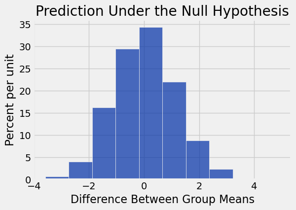
differences = np.append(differences, new_difference)Table().with_column('Difference Between Group Means', differences).hist()
print('Observed Difference:', observed_difference)
plots.title('Prediction Under the Null Hypothesis');Observed Difference: -9.266142572024918
Randomized Control Experiment
botox = Table.read_table('bta.csv')
botox.show()
Loading...
botox.pivot('Result', 'Group')Loading...
botox.group('Group', np.average)Loading...
Testing the Hypothesis
observed_diff = difference_of_means(botox, 'Result', 'Group')
observed_diff0.475one_simulated_difference(botox, 'Result', 'Group')-0.3simulated_diffs = make_array()
for i in np.arange(10000):
sim_diff = one_simulated_difference(botox, 'Result', 'Group')
simulated_diffs = np.append(simulated_diffs, sim_diff)col_name = 'Distances between groups'
Table().with_column(col_name, simulated_diffs).hist(col_name)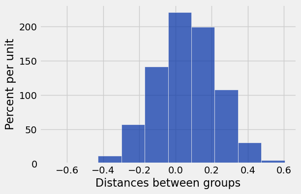
# p-value
sum(simulated_diffs >= observed_diff)/len(simulated_diffs)0.0063Discussion Question: Super Soda
def simulate_one_count(sample_size):
    return np.count_nonzero(np.random.choice(['H', 'T'], sample_size) == 'H')
simulate_one_count(200)100num_simulations = 10000
counts = make_array()
for i in np.arange(num_simulations):
counts = np.append(counts, simulate_one_count(200))trials = Table().with_column('Number of Heads', counts)
trials.hist(right_end=91)
plots.ylim(-0.001, 0.055)
plots.scatter(91, 0, color='red', s=40, zorder=3)
plots.title('Prediction Under the Null');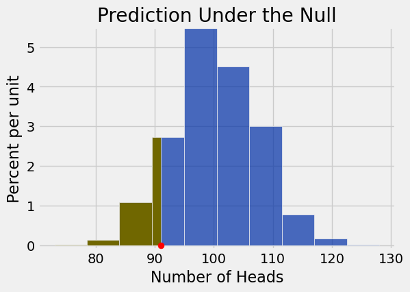
np.count_nonzero(counts <= 91)/len(counts)0.1117Conclusion:
Changing the number of simulations
# Keeping the data fixed, we can re-run the test with a new simulation under the null
def run_test(num_simulations, sample_size):
    counts = make_array()
    for i in np.arange(num_simulations):
        counts = np.append(counts, simulate_one_count(sample_size))
    return counts

counts = run_test(10000, 200)
np.count_nonzero(counts <= 91)/len(counts)0.1131# Let's repeat that 50 times for each number of simulations
tests = Table(['simulations', 'p-value for 91'])
for num_sims in [100, 1000, 10000]:
for k in np.arange(50):
counts = run_test(num_sims, 200)
tests = tests.with_row([
num_sims,
np.count_nonzero(counts <= 91)/len(counts),
])
tests.show(3)Loading...
# For larger numbers of simulations, p-values are more consistent
tests.hist(1, group='simulations')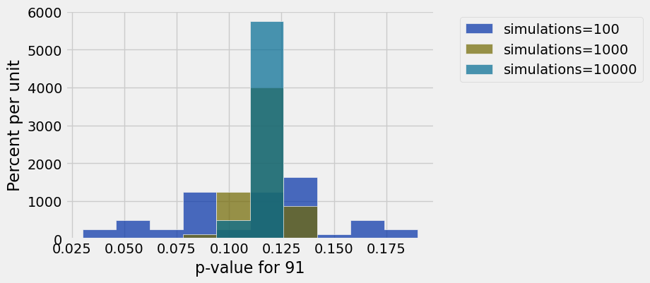
Changing the size of the taste test
# Suppose that the true proportion of people who prefer Super Soda is 45%
true_proportion = 0.45
true_distribution = make_array(true_proportion, 1 - true_proportion)
true_distribution
array([ 0.45, 0.55])# Taste tests with 200 people will give varioius numbers of people who prefer Super Soda
sample_size = 200
sample_proportions(sample_size, true_distribution) * sample_sizearray([ 77., 123.])# If you run a taste test for 200 people, what might you conclude?
def run_experiment(num_simulations, sample_size, true_proportion):
# Collect data
true_distribution = make_array(true_proportion, 1 - true_proportion)
taste_test_results = sample_proportions(sample_size, true_distribution) * sample_size
observed_stat_from_this_sample = taste_test_results.item(0)
# Conduct hypothesis test
counts = run_test(num_simulations, sample_size)
p_value = np.count_nonzero(counts <= observed_stat_from_this_sample) / len(counts)
return p_value
run_experiment(10000, 200, 0.45)0.4702# Let's imagine running our taste test over and over again to see how often we reject the null
true_proportion = 0.45
sample_size = 200
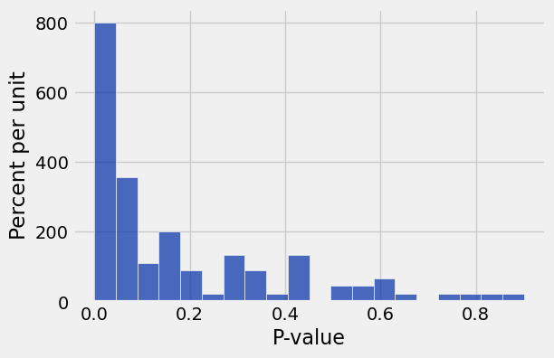
p_values = make_array()
for k in np.arange(100):
p_value = run_experiment(1000, sample_size, true_proportion)
p_values = np.append(p_values, p_value)
Table().with_column('P-value', p_values).hist(0, bins=20)
print('Percent of p-values at or below 0.05:', 100 * np.count_nonzero(p_values <= 0.05) / len(p_values))Percent of p-values at or below 0.05: 40.0